MPPT Charge Controller: How They Work and How to Select One

Introduction

Here is a failure pattern that is less dramatic than a tripped inverter or a discharged battery but equally costly over the life of a system. The array is correctly sized. The battery bank is correctly sized. The wiring is clean and the fusing is correct. The system runs without faults and the client has no complaints. But the daily energy harvest is consistently 15 to 20 percent below what the system should be producing based on the irradiance data for the site. No alarm triggers. No fault code appears. The system simply delivers less energy than it should, every day, for years.

In the cases I have investigated with this pattern, the MPPT charge controller is the bottleneck more often than any other component. Not because it is faulty, but because it was selected as a commodity purchase based on price and a single headline specification, typically the rated input voltage, without verifying the output current rating against the array, the thermal derating behavior in the installation environment, the charge algorithm compatibility with the battery chemistry, or the BMS communication capability of the specific model.

MPPT controller selection is not a commodity decision. It is a system-level engineering choice that affects every watt of energy the array produces from the first day of commissioning through the end of the system’s service life. In this post I am going to show you exactly which specifications matter, what they mean in practice, and how to evaluate them correctly.

How MPPT Tracking Actually Works

To select an MPPT controller intelligently, you need to understand what it is actually doing at an electrical level, because the specifications that matter most are directly connected to how well the controller executes its core function. That function is to find and continuously hold the operating point on the solar panel’s I-V curve where output power is maximized.

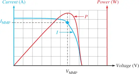
Every solar panel has an I-V curve that describes the relationship between its terminal voltage and output current under a given set of irradiance and temperature conditions. At one extreme of the curve, the panel is at open circuit: voltage is at its maximum Voc and current is zero, so power is zero. At the other extreme, the panel is short-circuited: current is at its maximum Isc and voltage is zero, so power is again zero. Somewhere between these two extremes is the maximum power point, the specific voltage and current combination where the product of the two is highest.

The formal relationship is:

P = V x I

Where:

P = panel output power (W)
V = panel terminal voltage (V)
I = panel output current (A)
Maximum power occurs at Vmp and Imp, where d(P)/d(V) = 0

The complication that makes MPPT non-trivial is that the maximum power point is not fixed. It shifts continuously as irradiance changes, as cell temperature changes, and as shading patterns change across the panel surface. At high irradiance and low cell temperature the MPP sits at a relatively high voltage and high current. As irradiance drops or cell temperature rises, the MPP shifts in both voltage and current simultaneously. The controller must track these shifts in real time to maintain maximum power extraction.

The algorithm most commonly used to track the MPP is called perturb-and-observe. The controller makes a small deliberate change to the operating voltage, observes whether output power increased or decreased as a result, and steps the voltage in the direction that increases power. It repeats this perturbation cycle continuously, oscillating around the true MPP. The step size and the cycle frequency of the perturbation determine how closely the controller tracks the true MPP and how quickly it responds to rapid irradiance changes.

The practical implication for controller selection is that tracking speed matters on sites with intermittent cloud cover. When a cloud edge passes over the array and irradiance changes rapidly, a controller with a slow perturbation cycle or a large step size will spend time hunting for the new MPP rather than delivering power at it. On a site with stable irradiance and clear skies, tracking speed is less critical. On a site with frequent cloud cover, a controller with fast dynamic MPPT response delivers measurably more daily energy harvest than a slow-tracking controller on the same array.

MPPT vs PWM: Why the Difference Matters in Practice

The performance difference between MPPT and PWM charge controllers is not a marketing distinction. It is a direct consequence of where each controller forces the solar array to operate on its I-V curve, and on any system where the array’s optimal operating voltage differs meaningfully from the battery voltage, the energy harvest difference between the two controller types is significant and measurable.

A PWM controller works by directly connecting the solar array to the battery through a switching element. When the battery needs charging, the switch closes and the array is connected directly to the battery bus. This forces the array to operate at the battery’s terminal voltage, which is typically between 24 and 58V on a 24V or 48V system depending on state of charge. If the panel’s Vmp is 38V and the battery terminal voltage is 27V, the PWM controller forces the array to operate at 27V instead of 38V, discarding the additional power the array could have delivered at its optimal operating point.

The energy harvest loss from PWM operation relative to MPPT on the same array can be estimated as:

PWM Harvest Loss (%) = (Vmp – Vbatt) / Vmp x 100

Example: Vmp = 38V, Vbatt = 27V
PWM Harvest Loss = (38 - 27) / 38 x 100 = 28.9%

That is a 29 percent reduction in energy harvest from the array simply from controller topology choice. An MPPT controller on the same system would operate the array at 38V, extract the full available power at that point, and then step the voltage down to the 27V charging voltage using its internal DC-DC converter, delivering the full available array power to the battery minus only the controller’s own conversion losses.

PWM controllers are only appropriate on small, simple systems where the panel voltage is already close to the battery charging voltage, specifically 12V nominal systems using panels designed for 12V direct charging. On any 24V, 48V, or higher voltage system using standard panels with a Vmp in the 30 to 42V range, PWM control represents a systematic and unrecoverable energy harvest loss that compounds every day for the life of the system.

DC-DC Converter Topology Buck vs Buck-Boost

The MPPT controller’s ability to operate the array at its optimal voltage and deliver charging current at a different voltage to the battery depends on its internal DC-DC converter. Understanding the two main converter topologies and when each applies is what allows you to evaluate whether a specific controller is correctly specified for your system’s voltage configuration.

A buck converter steps input voltage down to a lower output voltage while stepping current up proportionally, maintaining power balance minus conversion losses. This is the correct topology for the vast majority of off-grid MPPT applications, where the array string voltage at the maximum power point is higher than the battery charging voltage. A 48V battery system charging to 58V absorption voltage with a string Vmp of 100V is a straightforward buck application. The controller steps 100V down to 58V, and the output current is approximately 100/58 times the input current, less conversion losses.

A buck-boost converter can handle input voltages both above and below the output voltage, stepping up when necessary and stepping down when necessary. This topology is relevant in two specific scenarios: systems where the string Vmp at low irradiance conditions during early morning or late evening may fall below the battery voltage, and systems with very short string configurations where nominal Vmp is close to the battery voltage. In practice, well-designed string configurations with adequate series panel counts rarely fall into this territory, and buck-boost controllers carry a cost and efficiency penalty relative to pure buck designs that is only justified when the input voltage range genuinely spans both sides of the output voltage.

DC-DC Topology Selection Reference:

a. Array Vmp always > Battery Voltage -> Buck converter (standard, most efficient)
b. Array Vmp may fall below Vbatt -> Buck-boost required
c. Vmp close to Vbatt at low irradiance -> Verify with morning Vmp calculation
d. Buck-boost penalty -> Higher cost, lower peak efficiency

The morning low-irradiance Vmp calculation is the same check used in string compliance verification in Post #5: apply the temperature coefficient to the low-temperature Vmp and confirm the result against the controller’s minimum input voltage specification. If the minimum input voltage of a buck controller is above the early morning string Vmp, the controller will not begin tracking until irradiance rises enough to bring string voltage above its minimum threshold, delaying the start of morning charging.

Output Current Rating: The Primary Sizing Constraint

The specification that most directly determines an MPPT controller’s capacity is not its input voltage range, not its peak efficiency figure, and not its physical size. It is the rated output current, which defines the maximum DC current the controller can continuously deliver to the battery at the system voltage. Every other controller specification either supports or constrains this figure, and sizing the controller correctly starts here.

The relationship between array STC rating, real-world derating, system voltage, and required controller output current is:

I_out_required = (P_array_STC x Derating Factor) / V_battery

Where:

I_out_required = minimum required controller output current (A)
P_array_STC = total array STC rated power (W)
Derating Factor = real-world array output fraction (e.g., 0.718)
V_battery = nominal battery system voltage (V)

Applying this to the worked example from Post #4. The array is 2,400W STC. The derating factor for the tropical installation is 0.718. The system voltage is 48V:

I_out_required = (2,400W x 0.718) / 48V = 1,723W / 48V = 35.9A

A 40A controller is sufficient for this array and system voltage combination with a small margin. A 60A controller provides a more comfortable margin and accommodates future array expansion without controller replacement. A 30A controller would clip production whenever real-world array output exceeds 1,440W, which on this installation would occur for several hours every clear day.

What makes output current the primary sizing constraint rather than input power is that the controller’s thermal design is built around the output current it must sustain, not the input power it receives. A controller that clips the array at its output current limit is operating correctly and within its thermal design envelope. A controller that is forced to deliver more than its rated output current is operating outside its design envelope and will either thermally derate, trigger protection, or fail prematurely.

The practical rule I apply when selecting a controller is to calculate the required output current from the derated array output as shown above, then select a controller rated at a minimum of 10 to 15 percent above that figure to provide thermal and expansion margin. On installations where future array expansion is planned, I size the controller to the final intended array size rather than the initial installation to avoid a controller replacement cost later.

Temperature Derating in Hot Climates

Temperature derating is the MPPT controller performance limitation that catches the most installations off guard in tropical and subtropical climates, because it operates in the worst possible direction: the controller delivers less than its rated output precisely during the hours when solar irradiance is highest and the potential for energy harvest is greatest.

Every MPPT controller is rated at its full output current at a specific ambient temperature, almost universally 25 degrees Celsius. Above a threshold temperature, typically between 40 and 45 degrees Celsius depending on the controller model, the controller’s internal thermal protection begins to reduce the output current linearly to keep junction temperatures within safe limits. The rate of derating varies by manufacturer and model, but a common profile is a 1 to 1.5 percent reduction in rated output current per degree Celsius above the derating threshold.

On a controller rated at 60A with a derating threshold of 40 degrees Celsius and a derating rate of 1.25 percent per degree Celsius, the output at 55 degrees Celsius ambient is:

I_derated = I_rated x (1 - Derating Rate x (T_ambient - T_threshold))
I_derated = 60A x (1 - 0.0125 x (55 - 40))
I_derated = 60A x (1 - 0.1875) = 60A x 0.8125 = 48.75A

At 55 degrees Celsius ambient, this controller delivers only 48.75A rather than its rated 60A, an 18.75 percent reduction in available charging current during the hottest hours of the day. On a tropical installation where enclosure temperatures routinely reach 50 to 60 degrees Celsius during peak production hours, this derating is not an edge case. It is the normal operating condition.

Controller Thermal Derating Reference:

T_ambient 25°C          -> 100% rated output (STC reference)
T_ambient 40 to 45°C   -> derating begins (threshold varies by model)
T_ambient 55°C          -> typically 75 to 85% of rated output
T_ambient 65°C          -> typically 60 to 75% of rated output

Unventilated enclosure  -> add 15 to 25°C above ambient air temperature

The practical mitigation steps I apply on every tropical installation are as follows. First, specify a controller with a rated output current of at least 125 to 130 percent of the calculated required output current from Section 4, providing headroom for thermal derating. Second, install the controller in a ventilated enclosure with at least 50mm of clearance on all sides for convective airflow. Third, avoid installing the enclosure in direct sunlight or in rooms that accumulate heat during the day. A controller installed in a shaded, ventilated space consistently outperforms the same model installed in an unventilated box in direct sun, even when both are in the same climate.

Multiple MPPT Inputs and Split Array Architecture

The decision to use multiple MPPT inputs rather than combining all strings into a single controller input is one of the most consequential array architecture decisions on any installation where the array is not perfectly uniform in orientation, tilt, shading exposure, or panel model. The energy harvest penalty for combining mismatched strings at a single MPPT input was covered in Post #5, and the solution to that penalty is always the same: separate MPPT inputs that track each string group independently.

Modern hybrid inverters in the 3kVA to 10kVA range commonly offer two independent MPPT inputs, each with its own input voltage window and output current rating. The key specification to verify when selecting a dual-input controller is whether each input is truly independently tracked, meaning each input runs its own perturb-and-observe algorithm against its own string, or whether the dual input is simply a parallel combiner that feeds a single tracking stage. The former eliminates mismatch losses. The latter does not.

The sizing methodology for a split array architecture is to treat each MPPT input as an independent controller and apply the output current sizing calculation from Section 4 to each input separately. If the east-facing roof section carries 1,200W of panels on a 48V system with a 0.718 derating factor, that input requires a minimum of 17.95A output current capability. If the west-facing section carries 1,200W under the same conditions, it requires the same. A dual-input controller with two independent 20A stages correctly serves this installation.

When the string groups are large enough that each requires a controller output current beyond what a dual-input hybrid inverter can provide per input, the correct solution is separate standalone MPPT controllers rather than attempting to combine strings. Two 60A controllers, one per array section, each independently tracking and feeding the same battery bank, consistently outperform a single oversized controller receiving a combined mismatched input on any installation where the two array sections see meaningfully different irradiance profiles across the day.

For a detailed treatment of how string mismatch at a combiner point reduces array output and how to design string groups to eliminate it, refer to our post on series vs parallel vs series-parallel solar array wiring.

BMS Communication and Dynamic Charge Limiting

The integration between the MPPT charge controller and the battery management system is the design element that most clearly separates a properly engineered lithium battery system from one that is simply assembled from compatible components. On a system without active BMS-to-controller communication, the controller charges to its programmed voltage setpoints regardless of what is happening at the cell level inside the battery. On a system with active communication, the BMS instructs the controller in real time to reduce charge voltage or current in response to cell-level conditions that the controller cannot see on its own.

The two dynamic charge parameters the BMS communicates to the controller are the Charge Voltage Limit and the Charge Current Limit. The CVL tells the controller the maximum voltage it is permitted to apply to the battery terminals at the current moment. The CCL tells the controller the maximum current it is permitted to deliver.

Both parameters are dynamic, meaning the BMS adjusts them continuously based on cell voltages, cell temperatures, state of charge, and the balance state of the pack. When a cell group approaches its maximum voltage threshold during bulk charging, the BMS reduces the CVL before the controller’s programmed absorption voltage is reached, preventing that cell group from being overcharged even if the other cell groups in the pack are not yet full.

On systems without this communication link, the controller charges to its programmed absorption voltage based on battery terminal voltage alone. Terminal voltage is not cell voltage. On a battery pack with any degree of cell imbalance, the cell group with the highest voltage will reach its maximum threshold before the terminal voltage reaches the programmed absorption setpoint. Without a CVL signal from the BMS to reduce the charge voltage, that cell group will be overcharged while the controller continues pushing current into the pack. This is a systematic and cumulative degradation mechanism on any lithium system operating without BMS communication.

The communication protocols that carry CVL and CCL between BMS and controller vary by manufacturer. CAN bus at 250kbps or 500kbps is the most common protocol on quality lithium battery systems. Modbus RTU over RS485 is used on some standalone BMS units. Proprietary protocols such as Victron’s VE.Can, Pylontech’s CAN protocol, and PACE BMS protocol are used on specific battery and inverter combinations. Before selecting an MPPT controller for a lithium battery system, I verify that the controller supports the specific communication protocol used by the BMS, not just that it claims generic lithium compatibility.

For a detailed treatment of CVL and CCL operation and how dynamic charge limits protect cell-level integrity, refer to our engineering post on CVL, CCL, and DCL dynamic battery limits in real-time systems and our analysis of BMS-inverter communication protocols in modern solar systems.

Charge Algorithm Configuration for LiFePO4

The charge algorithm programmed into the MPPT controller is the configuration element that most installers set once during commissioning and never revisit, which is a problem when the default settings are built around lead-acid chemistry and the battery is LiFePO4. Getting this configuration wrong does not produce an immediate fault. It produces a systematic overcharge condition that degrades cell capacity gradually over hundreds of cycles, and by the time the capacity loss is noticeable the damage is already done.

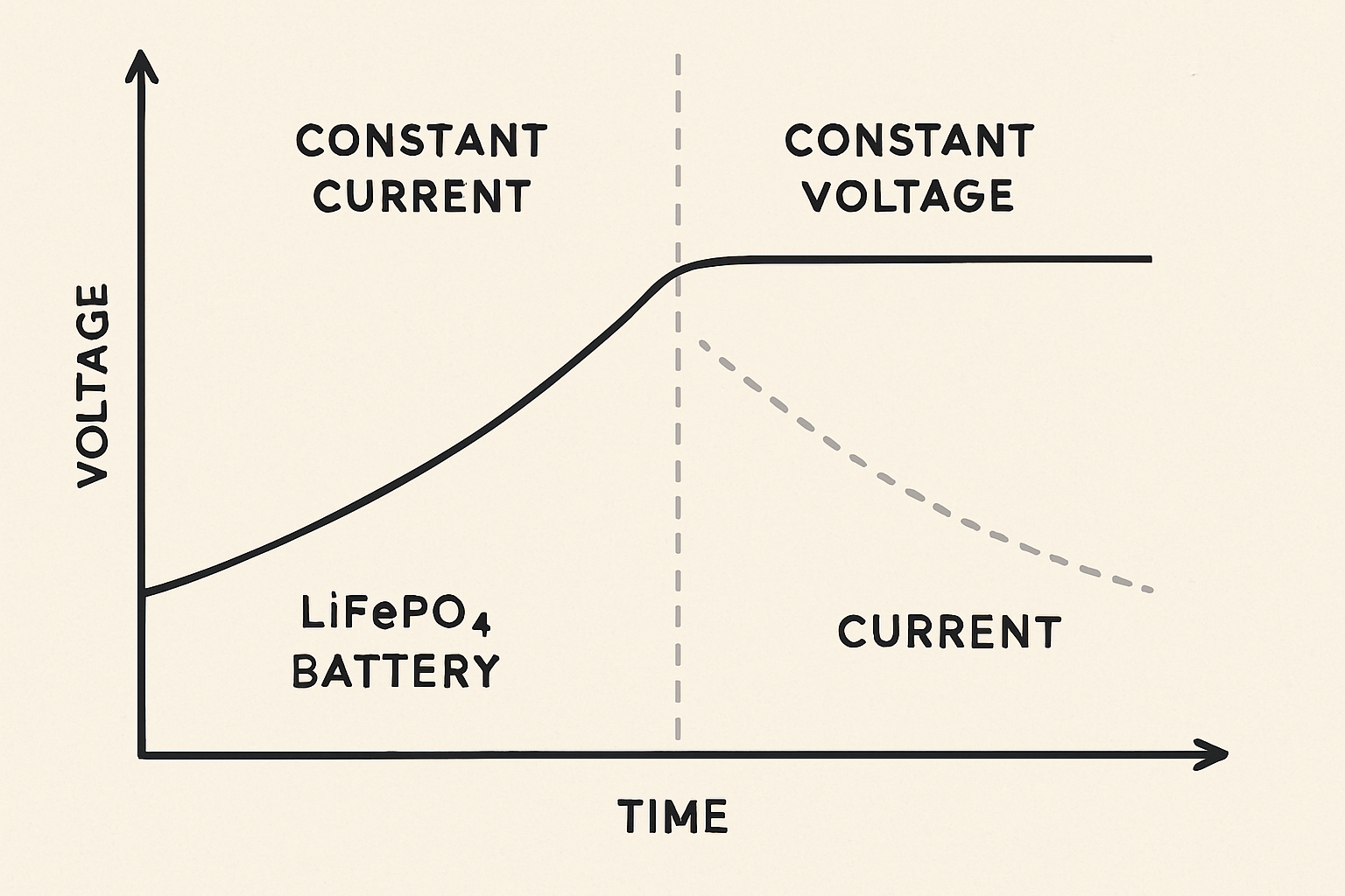
The correct charge algorithm for LiFePO4 is a two-stage constant current, constant voltage profile. In the bulk phase, the controller delivers maximum available current from the array at a constant rate until the battery terminal voltage reaches the absorption setpoint, typically 3.50 to 3.65V per cell, or 56V to 58.4V on a 16-cell 48V LiFePO4 pack. In the absorption phase, the controller holds the terminal voltage at the absorption setpoint and allows current to taper naturally as the cells approach full charge. Charging is considered complete when the current tapers below a defined threshold, typically 2 to 5 percent of the battery’s rated capacity in ampere-hours.

LiFePO4 Charge Parameter Reference (48V / 16-cell system):

Absorption voltage-> 56.0V to 58.4V  (3.50V to 3.65V per cell)
Float voltage -> 54.4V to 55.2V  (3.40V to 3.45V per cell)

Float rule -> must be BELOW absorption voltage

Absorption end current -> 2 to 5% of battery Ah rating

Equalization -> DISABLED, always

Three-stage profile -> acceptable only if float correctly set below absorption

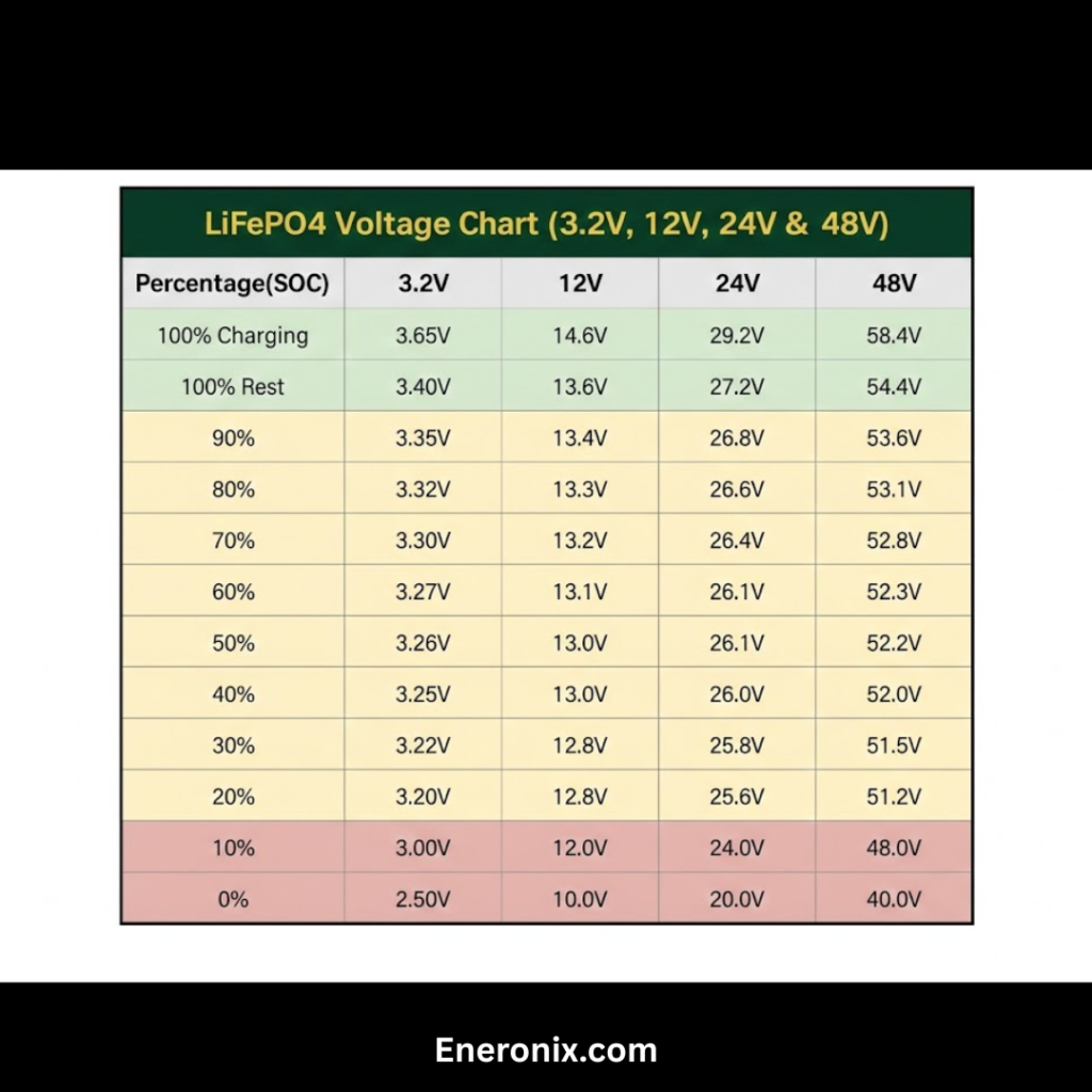
The float voltage setting requires particular attention. A float voltage set at or above the absorption voltage means the controller will continuously hold the battery at full charge voltage indefinitely after the charging cycle completes, which constitutes a chronic low-level overcharge condition. The correct float voltage for LiFePO4 is set below the absorption voltage, typically at 3.40 to 3.45V per cell, which allows the battery to rest at a partial state of charge between charging cycles rather than being held continuously at maximum voltage.

LiFePO4 Configuration Checklist:

1. Absorption voltage -> verify with battery manufacturer datasheet
2. Float voltage -> must be below absorption voltage
3. Equalization -> disabled
4. Absorption timeout -> set to minimum or current-taper termination
5. BMS communication -> active CVL overrides programmed setpoints if connected

Reading Efficiency Curves and Real-World Performance

The peak efficiency figure published in an MPPT controller’s datasheet is the number that appears most prominently in marketing materials and comparison tables, and it is the least useful single number for predicting real-world system performance. Peak efficiency is measured at a specific and favorable combination of input voltage, output power level, and ambient temperature that represents the best-case operating condition for that controller. The question that matters for system design is not what the controller achieves at its best-case operating point, but what it achieves across the full range of conditions it will actually experience during a typical day.

A typical off-grid system charges its battery from near-empty to full across a solar day that begins with low irradiance at sunrise, rises to peak irradiance at solar noon, and falls back to low irradiance at sunset. During the morning and evening low-irradiance periods, the array is producing at 20 to 40 percent of its peak output, the controller is operating at partial load, and its efficiency drops meaningfully below the peak figure. A controller with a published peak efficiency of 98 percent may operate at 93 to 94 percent efficiency during these partial-load periods.

The correct way to compare two controllers on efficiency is to examine the full efficiency curve across the output power range, not just the peak figure. Most quality controller manufacturers publish these curves in the datasheet. The comparison that matters is efficiency at 20 percent of rated output, at 50 percent of rated output, and at 100 percent of rated output. A controller that shows 96 percent efficiency at 20 percent load is more valuable in practice than one that shows 98 percent at 100 percent load but drops to 90 percent at 20 percent load, because on most days the controller spends more cumulative time at partial load than at full rated output.

Load Level	Controller A	Practical Significance
20% rated output	90%	Morning / evening harvest — high hours per day
50% rated output	95%	Cloud cover and shoulder hours
100% rated output	98%	Peak midday — fewer hours per day

The real daily harvest impact of a 2 to 3 percent efficiency gap across partial-load operating periods is calculable. On a system harvesting 10kWh per day with 30 percent of that harvest occurring during partial-load conditions, a 3 percent efficiency gap at partial load costs 0.09kWh per day, or approximately 33kWh per year. Over a 10-year system life, that gap represents 330kWh of undelivered energy from a single specification choice that most designers never examine beyond the headline peak efficiency figure.

Conclusion

MPPT charge controller selection sits at the intersection of every major design decision in an off-grid system. It receives the array output that Post #4 sized and Post #5 configured. It feeds the battery bank that must sustain the loads the first three posts quantified. It communicates with the BMS that protects the cells. It executes the charge algorithm that determines how the battery is treated across thousands of cycles. A controller selected as an afterthought or a cost-saving measure undermines the engineering that went into every other component in the system.

The specifications that determine real-world controller performance are, in order of importance: rated output current matched to the derated array output at the system voltage, thermal derating behavior at the installation’s actual ambient temperature, BMS communication protocol compatibility with the specific battery system, charge algorithm configurability for LiFePO4 chemistry, and efficiency across the partial-load range rather than just at the peak rated point. These are the five questions I answer before selecting any MPPT controller for a lithium battery system.

What the worked examples in this post demonstrate consistently is that a controller sized to 125 to 130 percent of the calculated required output current, installed in a ventilated enclosure, communicating with the BMS via the correct protocol, and configured with correct LiFePO4 charge parameters will deliver measurably more energy to the battery every day than a nominally higher-rated controller that fails on any one of those criteria.

In the next post in this series we will build a complete MPPT controller selection worked example using the array and system parameters established across Posts #4 and #5, selecting a specific controller configuration and verifying every specification against the system requirements.

For the array sizing and string configuration methodology that feeds the controller sizing calculations in this post, refer to our engineering guides on how to size a solar array for an off-grid lithium battery system and series vs parallel vs series-parallel solar array wiring.